
How to Use VLOOKUP in Excel: A Step-by-Step Guide (2026)
Imagine manually scrolling through thousands of rows of data just to find the price of a single item. It’s tedious, prone to errors, and a massive waste of time. Enter VLOOKUP—one of Excel’s most powerful and popular functions.
Short for “Vertical Lookup,” VLOOKUP acts like a digital search engine for your spreadsheets. You give it a piece of information (like a Product ID), and it searches a list to return corresponding details (like a Price) from the same row. Whether you are managing inventory, analyzing sales data, or organizing a massive contact list, mastering VLOOKUP can turn hours of manual work into seconds of automated magic.
The Syntax: How VLOOKUP Speaks
To use VLOOKUP, you need to tell Excel four specific things. The formula looks like this:
=VLOOKUP(lookup_value, table_array, col_index_num, [range_lookup])
Here is what that actually means in plain English:
- Lookup_value (What are you looking for?): This is the specific item you want to find. It is usually a unique identifier, like an ID number or a name.
- Table_array (Where should I look?): This is the range of cells that contains your data. Important: The first column of this range must contain the Lookup_value.
- Col_index_num (Which column has the answer?): This is the column number in your table that contains the data you want to retrieve (e.g., Column 3 for Price).
- [Range_lookup] (Do you want an exact match?): This tells Excel if you want the exact item or something “close enough.”
- FALSE (or 0): Gives you an Exact Match. (Recommended for most beginners).
- TRUE (or 1): Gives you an Approximate Match.
Real-World Example: Finding Product Prices
Let’s say you manage a small coffee shop inventory. You have a list of products with their IDs, names, and prices. You want to quickly find the Price of a specific item using its Product ID.
Here is your data set (Table A):
| Row | A (Product ID) | B (Product Name) | C (Price) |
| 2 | 101 | Espresso Roast | $15.00 |
| 3 | 102 | Vanilla Syrup | $8.50 |
| 4 | 103 | Paper Cups (50pk) | $12.00 |
| 5 | 104 | Almond Milk | $4.50 |
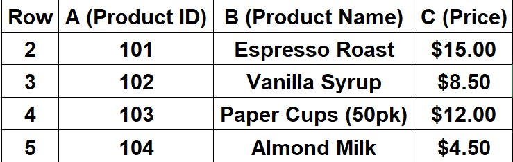
The Goal: You want to type the Product ID 103 into cell E2 and have Excel automatically populate the Price in cell F2.
Step-by-Step Tutorial
Follow these steps to write your first VLOOKUP formula based on the example above.
- Click the cell where you want the answer: Click on cell F2 (this is where the price will appear).
- Start the formula: Type
=VLOOKUP( - Enter the Lookup Value: Click on cell E2 (where you typed the ID 103). Add a comma.
- Formula so far:
=VLOOKUP(E2,
- Formula so far:
- Select the Table Array: Highlight your entire data table from A2 to C5. Add a comma.
- Formula so far:
=VLOOKUP(E2, A2:C5,
- Formula so far:
- Enter the Column Index Number: Count the columns from left to right. Product ID is Col 1, Name is Col 2, and Price is Col 3. Since we want the Price, type 3. Add a comma.
- Formula so far:
=VLOOKUP(E2, A2:C5, 3,
- Formula so far:
- Choose Exact Match: Type FALSE (or 0) because you want the exact price for ID 103, not a similar one. Close the parenthesis.
- Final Formula:
=VLOOKUP(E2, A2:C5, 3, FALSE)
- Final Formula:
- Press Enter: Excel will look for ID 103, go to the 3rd column, and display $12.00.
Common Errors: Why am I seeing #N/A?
The most common error users face is the dreaded #N/A error. This usually means “Not Available,” and it happens for a few specific reasons:
- The value doesn’t exist: You searched for “108”, but your list only goes up to “104”.
- The formatting is different: Your Lookup Value is stored as Text, but the table data is stored as a Number (or vice versa). Excel sees these as two different things.
- Missing “FALSE”: If you forget to type FALSE at the end of your formula, Excel defaults to “Approximate Match.” If your list isn’t sorted in ascending order, this can return the wrong result or an error.
FAQ: Common Questions About VLOOKUP
1. Can VLOOKUP look to the left?
No. This is VLOOKUP’s biggest weakness. It can only look for a value in the first column of your range and return data from columns to the right. If you need to look left, you should look into using XLOOKUP or the INDEX/MATCH combination.
2. What happens if I insert a new column in my table?
If you insert a column between A and C, your “Price” column is no longer the 3rd column; it becomes the 4th. VLOOKUP does not update automatically, so your formula will break or return the wrong data. You will need to manually change the column index number in your formula.
3. Is VLOOKUP case-sensitive?
No. VLOOKUP treats “apple”, “APPLE”, and “Apple” exactly the same way.
Conclusion
Congratulations! You have just unlocked one of the most essential skills in data management. While it might seem intimidating at first, VLOOKUP is straightforward once you understand the four parts of the syntax. Start by practicing with small tables like the one in this guide. Before long, you’ll be cross-referencing massive datasets with confidence and saving yourself hours of manual work.
Happy Spreadsheeting!